Differences in Equity Sector and Government Bond Comovement
For the last four decades, stock-bond correlations have moved quite a bit. However, for the better part of the last two decades, they have remained largely negative, even if noisily so. This has been beneficial to owners of traditional 60-40 funds.
Depending on the securities one chooses as a proxy for stocks and bonds, we have seen a relatively dramatic move from negative to positive correlations in the last few years. This has been relatively painful, particularly during 2022, for 60-40 investors. Equity and bond markets went down in tandem providing a one-two punch to the chin.
Choosing securities readily available to retail investors makes the point. We can choose the iShares Russell 1000 ETF (IWB) and iShares 7-10 Year Treasury Bond ETF (IEF) to represent the equity and bond markets, respectively.
Computing rolling one year correlations between IWB and IEF results in the chart shown in Figure 1.
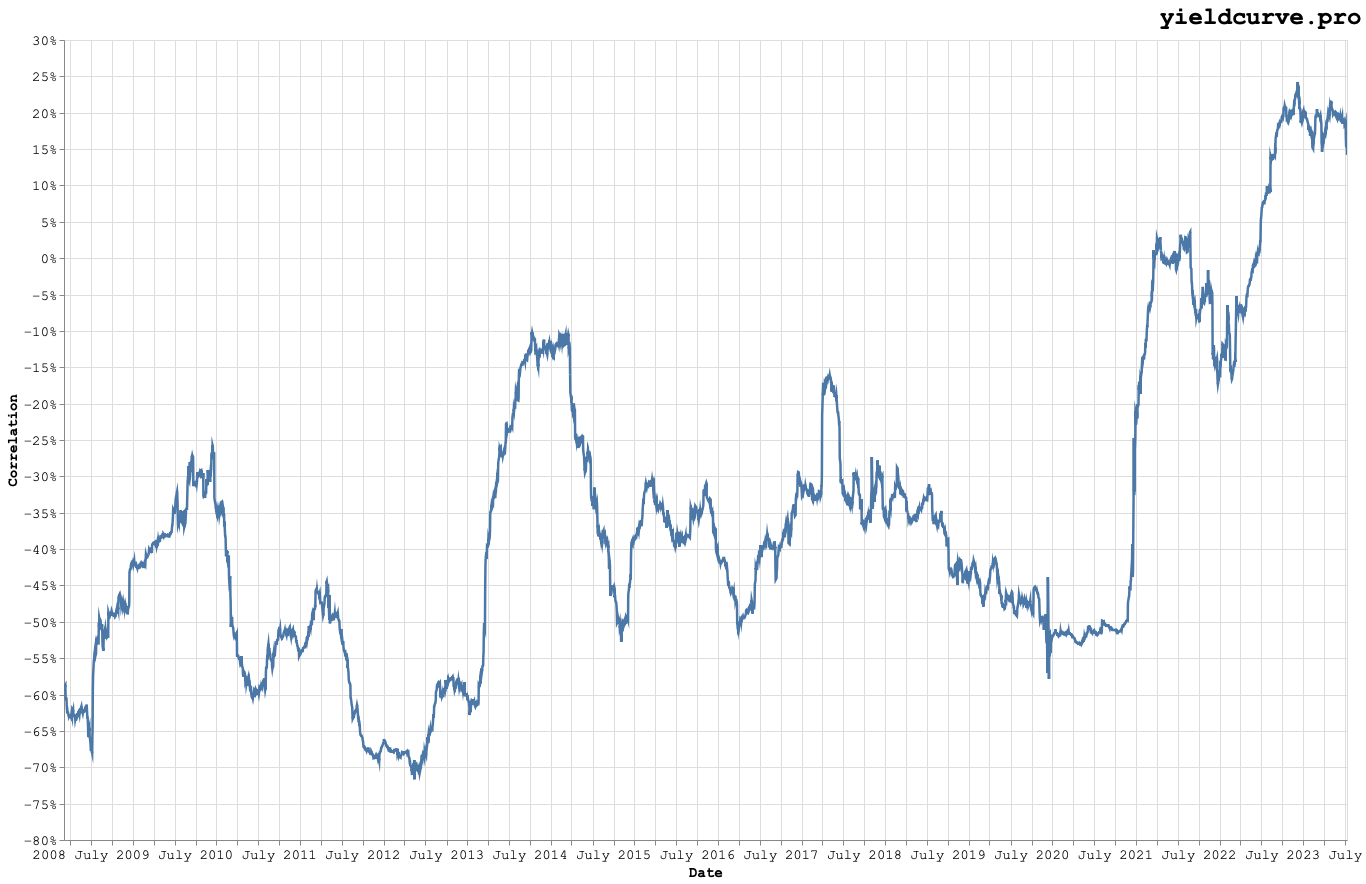
Figure 1: Rolling Equity (IWB) and Bovernment Bond (IEF) Correlations.
This chart should make clear both the noisiness in correlations as well as the pain 60-40 investors have been experiencing the last few years. If it's not apparent looking at correlations then it should clear looking at the wealth curves shown in Figure 2. While the equity markets have exhibited corrections similar to many we have seen in the past the bond markets have experienced sharp and uncharacteristic drawdowns.
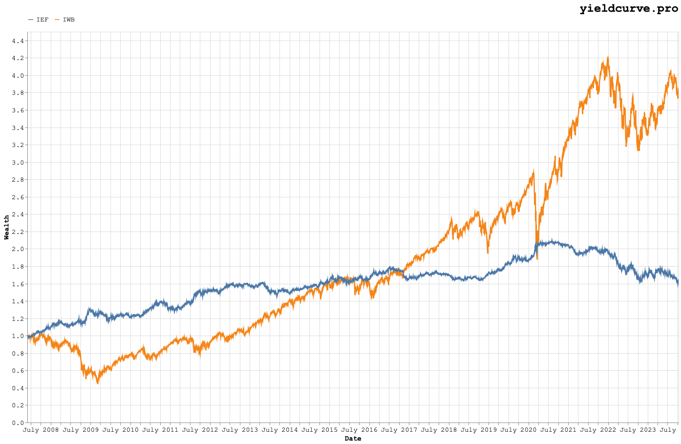
Figure 2: Equity (IWB) and Government Bond (IEF) Wealth Curves.
Together, these raise some interesting questions. Considering how the positive correlations (or comovements) in stocks and bonds have thrashed 60-40 funds recently, investors might wonder how consistently they hold for subsets of the equity market. Specifically, is there dispersion (or not) in the comovement between the GICS (the sectors comprising the equity market) and government bonds?
We follow existing work 1,2 that attempts to explain asset excess returns using a multivariate regression of the form shown in Equation 1.
$$ r_{st} - r_f = \alpha_s + \beta_{m}\left(r_{mt} - r_f\right) + \beta_{b}\left(r_{bt} - r_f\right) + \epsilon_{st} \qquad\qquad\qquad\qquad (1) $$ where $$r_{st} := \text{sector return}$$ $$r_{mt} := \text{stock market return}$$ $$r_{bt} := \text{bond market return}$$ $$r_f := \text{risk free rate}$$ $$\alpha_s := \text{intercept}$$ $$\beta_{m} := \text{stock market exposure}$$ $$\beta_{b} := \text{bond market exposure}$$
Table 1 shows the sector ETFs we use to represent our investible universe.
| Ticker | Description |
|---|---|
| XLC | Communication Services |
| XLY | Consumer Discretionary |
| XLP | Consumer Staples |
| XLE | Energy |
| XLF | Financials |
| XLV | Health Care |
| XLI | Industrials |
| XLB | Materials |
| XLRE | Real Estate |
| XLK | Technology |
| XLU | Utilities |
Table 1: Sector ETF Universe
For simplicity, and keeping with our preference for using securities easily avaiable to retail investors, we use the SPDR Bloomberg 1-3 Month T-Bill ETF (BIL) as our proxy for the risk free rate. But "wait!" you might protest, that isn't risk free at all. In fact, that ETF loses money on occasion. Well, we at yieldcurve.pro tend to the lazy side and hand wave that inconvenient fact away with the following reasoning: it's close enough and that's the best we unsophisticated retail investors can do.
Table 1 shows excess returns, volatilities, and information ratio (IR) over the entire period.
| Ticker | Description | Excess Return (%) | Excess Volatility (%) | IR |
|---|---|---|---|---|
| IEF | 7-10 Year Treasury | 2.43 | 7.12 | 0.34 |
| IWB | Russell 1000 | 9.62 | 20.53 | 0.47 |
| XLC | Communication Services | 8.26 | 24.67 | 0.33 |
| XLY | Consumer Discretionary | 11.97 | 23.44 | 0.51 |
| XLP | Consumer Staples | 8.54 | 15.37 | 0.56 |
| XLE | Energy | 8.95 | 31.96 | 0.28 |
| XLF | Financials | 6.88 | 32.24 | 0.21 |
| XLV | Health Care | 10.51 | 18.35 | 0.57 |
| XLI | Industrials | 9.78 | 22.66 | 0.43 |
| XLB | Materials | 8.58 | 24.83 | 0.35 |
| XLRE | Real Estate | 6.14 | 21.50 | 0.29 |
| XLK | Technology | 15.06 | 23.37 | 0.64 |
| XLU | Utilities | 6.86 | 20.01 | 0.34 |
Table 2: Bond, Stock, and Sector Index Summary Statistics (Annualized)
Generally speaking, IR implies active managment. Since these numbers are simply in excess of the risk free rate one should not take the IR's too seriously.
The parameters in Equation 1 are estimated using daily returns and 256 day rolling windows. Why 256? Two exceedingly good reasons: its square root is 16 (which is easy to remember when annualizing) and recall that we're lazy. Turning the analytical crank and Figures 3, 4, and 5 are what fall out.
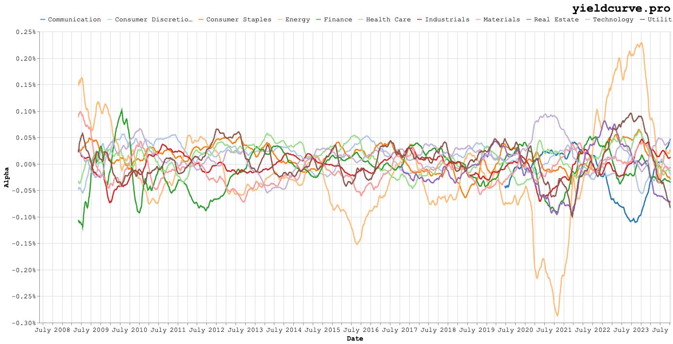
Figure 3: Rolling Alpha (Intercept) Term by Sector
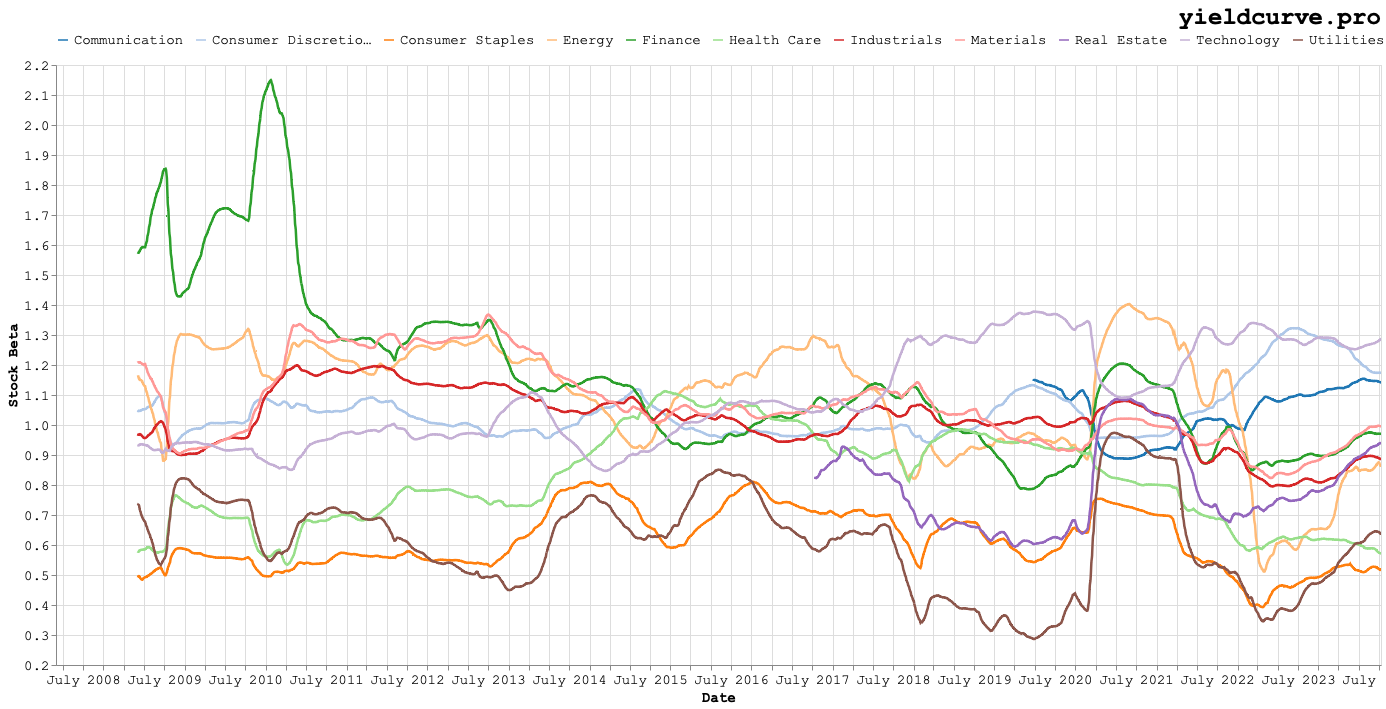
Figure 4: Rolling Stock Beta by Sector
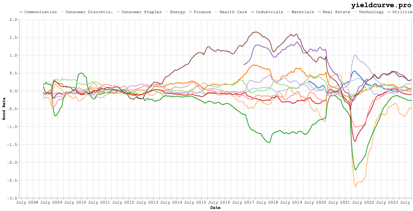
Figure 5: Rolling Bond Beta by Sector
Figures 3 and 4 are fun to look at but don't really reveal too many things to the naked eye. Figure 5, on the other hand, shows increasing dispersion in bond beta around 2013. Things get even more interesting as 2017 approaches and continues to the current period.
Between 2013 and 2020, the upper and lower extremes in dispersion are caused by Utilities and Financials, respectively. From 2020 on, the lower bound is dominated by the Energy and Financial sectors. While we can speculate on what is happening by visual inspectin of the charts, perhaps a table of averages can make empirical comparisons more straightforward.
Table 3 shows average values for the esimated regression parameters.
| Ticker | Sector | Alpha (Annualized %) | Stock Beta | Bond Beta |
|---|---|---|---|---|
| XLC | Communication | -4.22 | 1.04 | 0.13 |
| XLY | Consumer Discretionary | 2.76 | 1.04 | 0.01 |
| XLP | Consumer Staples | 3.05 | 0.61 | 0.17 |
| XLE | Energy | -4.04 | 1.09 | -0.28 |
| XLF | Finance | -2.51 | 1.15 | -0.51 |
| XLV | Health Care | 2.86 | 0.81 | 0.09 |
| XLI | Industrials | -0.92 | 1.02 | -0.17 |
| XLB | Materials | -2.87 | 1.07 | -0.08 |
| XLRE | Real Estate | -2.81 | 0.79 | 0.72 |
| XLK | Technology | 4.11 | 1.09 | 0.10 |
| XLU | Utilities | 1.83 | 0.61 | 0.55 |
Table 3: Average Multivariate Regression Parameters by Sector
We can cherry pick a few interesting things that stand out. The Communication (XLC) and Technology (XLF) sectors sit on opposite sides of the Alpha specturm while maintaining very similar exposures to Stock and Bond Beta. What is more interesting is the dispersion in Bond Beta across sectors. Could timing these provide a way to construct more durable 60-40 portfolios with better risk-adjusted returns? Perhaps.
Examining the time varying characteristics of Bond Beta could be an interesting area for further research. Another interesting aspect of this analysis is its ability to suggest asset classes that could be additive to an existing stock-bond allocation (be it 60-40 or something else entirely). How is this useful? By selecting those assets that are additive on an Alpha basis while providing as little exposure to your chosen stock and bond indices. This provides a nice framework to answer questions like:
- Do commodities add anything to this allocation?
- Should I add corporate debt or is that just doubling down on the leveraged equity bet I already have?
All interesting questions and ones that will need to wait for a subsequent blog post.
Back