The 10 Yr Yields 5.29%. The Curve Still Says Hold Bills.
On September 30, 2026, the 10 Yr yield closed at 5.29%, its highest close since May 2002. Over the previous twelve months, a constant 10 Yr Treasury position lost 4.05%. A 30 Yr position lost 8.59%. Rolling 1 Mo bills earned 3.90%. An investor holding bills now has to decide whether yields this high justify buying longer maturities.
A 1995 study addresses that decision. In Part 3 of Understanding the Yield Curve, a Salomon Brothers research series, Antti Ilmanen tested whether investors earn more over the long run by extending duration beyond bills. All seven parts are free to read in the yieldcurve.pro library of classic fixed income papers. Earlier posts covered Part 1 and Part 2.
In February 2024, the asset manager Cambria Investment Management proposed a rule for when to sell bills and buy longer duration bonds in T-Bills and Chill... Most of the Time. This post reruns Ilmanen's test and Cambria's rule on current data.
What Ilmanen tested
Ilmanen measured the extra return a Treasury holder earns, over many years, for holding a longer maturity. He called it the bond risk premium. This post calls it the excess return, which is the return of a maturity minus the return of a short bill.
He chose 1970-1994 because yields at the start and end of that period were comparable. A bond's average excess return is approximately its average yield in excess of bills minus its duration times the average change in its yield. Duration is the percentage change in a bond's price for a one-point change in its yield. When yields end where they started, the average change is near zero. The average excess return then measures the premium the market offered.
Most of the premium he found was at the front of the curve. A 1 Yr bill earned about 1.5% a year more than a 1 Mo bill. Beyond 2 Yr, he found no clear extra return. He also found that a steep curve at the start of a month predicted high 20 Yr bond returns over that month.
Data and a check against the 1995 numbers
We use two data sets. The Treasury par yield curve covers every maturity from 1 Mo to 30 Yr since July 2001, which gives 302 monthly returns. Yields in that sample also end near where they started, as Ilmanen required. The 20 Yr yield went from 5.61% to 5.68%, and the 1 Mo yield went from 3.67% to 4.02%. The second data set, the Federal Reserve's constant maturity yields on FRED, covers the 3 Mo bill and the 1, 3, 5 and 10 Yr back to 1962. It gives 776 monthly returns.
Treasury stopped issuing the 30-year bond from February 2002 to February 2006 and published no 30 Yr yield in those years. The 30 Yr statistics therefore cover its 253 quoted months, not 302.
We compute monthly returns from the yield curve. At the start of each month, we buy each maturity at its current yield. At the end of the month, we sell it. A 10 Yr bond sold after one month has 9 years and 11 months left, so we price it at the end-of-month yield for that maturity. On an upward-sloping curve, that yield is a little lower than the 10 Yr yield, which adds a small price gain called the roll-down return.
As a first check, we compare these returns with six Treasury exchange-traded funds (ETFs), matching each fund to the maturity closest to its holdings. The correlation of monthly returns ranges from 0.96 for our 1 Mo bill against a T-bill fund (BIL) to 0.995 for our 5 Yr against a 3-7 Yr Treasury fund (IEI).
Table 1 rebuilds Ilmanen's 1970-1994 sample from the FRED data and compares it with his published numbers.
| Maturity | Our average yield | Ilmanen's | Our compounded return | Ilmanen's (bucket) |
|---|---|---|---|---|
| 3 Mo | 7.22% | 7.21% | 7.37% | 7.71% (3 Mo bill) |
| 1 Yr | 7.76% | 7.73% | 8.63% | 8.52% (1-2 Yr) |
| 3 Yr | 8.25% | 8.18% | 9.12% | 8.95% (3-4 Yr) |
| 5 Yr | 8.47% | 8.44% | 9.12% | 8.82% (4-5 Yr) |
| 10 Yr | 8.70% | 8.63% | 9.09% | 8.98% (5-10 Yr) |
Table 1: Average yield and compounded annual return, 1970-1994, our rebuild from FRED against Ilmanen's Figures 3 and 5. His bond returns are for maturity buckets, ours for single maturities.
Average yields match within 0.07 percentage points, and bond returns within 0.30 points. Our 3 Mo bill earns 0.34 points less than his. FRED has no bill shorter than 3 Mo before 2001, so our 3 Mo bill earns only its yield, with no price gain from aging.
The premium for longer bills has disappeared
Ilmanen's strongest result was the extra return on longer bills over the 1 Mo bill. The yield gap between two bills measures the premium the market offers for the longer bill before rates move. It gives the cleanest test of whether his result survives.
In 1970-1994, the 3 Mo bill yielded 0.46 percentage points more than the 1 Mo bill on average. In 2001-2026, it yielded 0.05 points more. The 1 Yr bill's advantage fell from 0.98 points to 0.21. Table 2 shows that realized excess returns are similarly small. Its t-statistics measure how far each average sits from zero in units of its sampling error. A value above 2 is the usual threshold for statistical significance.
| Months starting with | Months | 3 Mo yield over 1 Mo | 3 Mo excess return | 1 Yr yield over 1 Mo | 1 Yr excess return |
|---|---|---|---|---|---|
| All months | 302 | +0.05% | +0.08% (t 3.71) | +0.21% | +0.28% (t 2.28) |
| 1 Mo below 1% | 147 | +0.04% | +0.04% (t 3.44) | +0.26% | +0.20% (t 1.71) |
| 1 Mo at 1% or more | 155 | +0.07% | +0.12% (t 2.84) | +0.16% | +0.36% (t 1.69) |
| 1 Mo at 4% or more | 60 | +0.03% | +0.02% (t 0.53) | -0.12% | -0.03% (t -0.10) |
Table 2: Average yield over the 1 Mo bill at the start of the month, and average annualized excess return over the 1 Mo bill, by the 1 Mo yield at the start of the month, August 2001 to September 2026.
Near-zero rates do not explain the decline. In months that began with the 1 Mo bill at 1% or more, the 3 Mo bill offered only 0.07 points of extra yield. In months that began at 4% or more, the 1 Yr bill yielded less than the 1 Mo bill on average. A bill curve inverted in this way usually reflects expected rate cuts. An investor holding idle cash in Treasury bills gains almost nothing by choosing longer bills.
The premium for longer bonds is positive but statistically weak
Table 3 shows each maturity from 2001 to 2026. The Sharpe ratio is the average excess return divided by its volatility, a measure of return per unit of risk.
| Maturity | Annual return | Excess over 1 Mo | Volatility | Sharpe ratio | t-statistic |
|---|---|---|---|---|---|
| 1 Mo | 1.74% | 0.00% | 0.53% | ||
| 3 Mo | 1.82% | +0.08% | 0.54% | 0.74 | 3.71 |
| 6 Mo | 1.98% | +0.24% | 0.58% | 0.90 | 4.50 |
| 1 Yr | 2.03% | +0.29% | 0.79% | 0.46 | 2.28 |
| 2 Yr | 2.30% | +0.56% | 1.62% | 0.36 | 1.82 |
| 3 Yr | 2.63% | +0.89% | 2.57% | 0.36 | 1.80 |
| 5 Yr | 3.35% | +1.61% | 4.35% | 0.38 | 1.92 |
| 7 Yr | 3.77% | +2.03% | 5.84% | 0.37 | 1.84 |
| 10 Yr | 3.80% | +2.06% | 7.62% | 0.30 | 1.51 |
| 20 Yr | 4.20% | +2.46% | 11.89% | 0.26 | 1.30 |
| 30 Yr | 2.63% | +0.90% | 15.14% | 0.13 | 0.61 |
Table 3: Compounded annual return, compounded excess return over the 1 Mo bill, annualized volatility, Sharpe ratio, and t-statistic of the average monthly excess return, August 2001 to September 2026. The 30 Yr row covers its 253 quoted months.
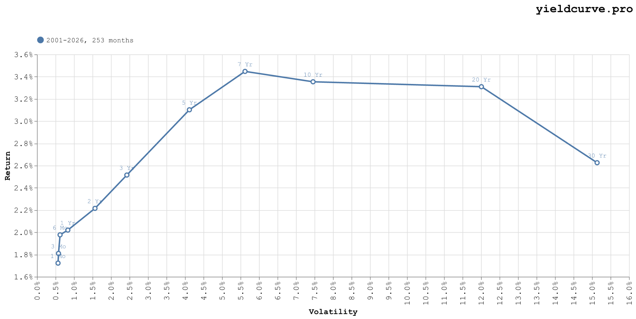
Figure 1: Compounded annual return against volatility for each maturity, over the 253 months from August 2001 to September 2026 in which the 30 Yr is quoted.
Every bond maturity earned more than bills, but no bond premium is statistically significant, because the sample is too short. With monthly data, a t-statistic is about the Sharpe ratio times the square root of the number of years. At a Sharpe ratio of 0.30, a t-statistic of 2 takes 44 years of data. At 0.13, it takes 237 years. Ilmanen faced the same limit. His 20 Yr bond had a Sharpe ratio of 0.22 over 25 years, which implies a t-statistic near 1.1.
The 64-year FRED sample can detect smaller premiums. Over 1962-2026, the excess return over the 3 Mo bill was +0.70% a year for the 1 Yr (t 4.69), +1.14% for the 3 Yr (t 2.71), +1.45% for the 5 Yr (t 2.29) and +1.79% for the 10 Yr (t 1.88). The premium rises with maturity at a falling rate. Even over 64 years, the 10 Yr premium falls short of significance.
Beyond 2 Yr, the 2001-2026 premium rises more steeply than Ilmanen's did. The difference is within sampling error. The 7 Yr beat the 2 Yr by 1.58% a year (t 1.73), and the 20 Yr beat the 7 Yr by 0.94% (t 0.67). All three samples fit a premium that rises with maturity and then flattens.
Return per unit of risk falls with maturity. The Sharpe ratio drops from 0.90 at 6 Mo to 0.36 at 2 Yr, stays near 0.37 out to 7 Yr, and falls to 0.13 at 30 Yr. The 30 Yr had more than two and a half times the volatility of the 7 Yr and a lower compounded return. Volatility pulls a compounded return below the average monthly return. The 30 Yr's average monthly return comes to 3.79% a year, but it compounded at 2.63%.
Figure 1 compares every maturity over the same 253 months, so the 30 Yr is measured against the same history as the rest. On those months the compounded return peaks at the 7 Yr (3.45%), edges down through the 10 Yr (3.35%) and the 20 Yr (3.31%), and falls at the 30 Yr (2.63%). The 20 Yr's higher return in Table 3 comes from the four years the 30 Yr was not quoted, when the 20 Yr compounded at 8.9% a year.
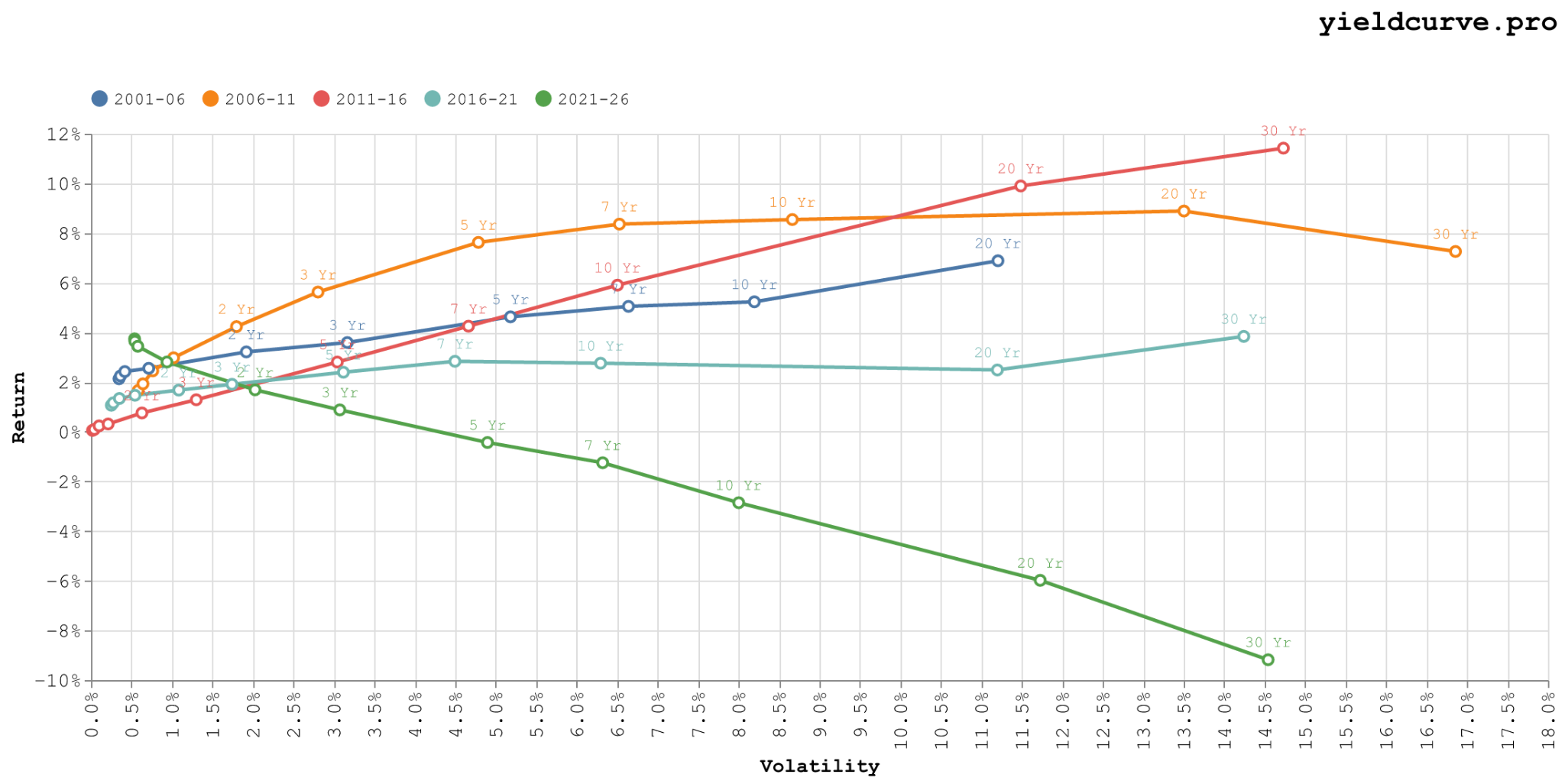
Figure 2: Compounded annual return against volatility in five subperiods. Labels mark maturities of 2 Yr and longer.
The premium also varies widely across subperiods (Figure 2). From 2011 to 2016, the 30 Yr returned 11.42% a year. From 2021 to 2026, it lost 9.18% a year. A long-run average this unstable gives little guidance on how much duration to hold today.
A steep curve predicts higher bond returns
Ilmanen found that the slope of the curve explains part of this variation. He sorted months by the 20 Yr yield minus the 1 Mo yield at the start of each month. He set his thresholds of 0 and 300 bp in 1995, before any of our 2001-2026 data existed. Applying them unchanged therefore tests the result on data that played no part in choosing it.
| Starting slope | Months | 20 Yr return | 20 Yr excess return |
|---|---|---|---|
| Below 0 bp | 31 | -1.97% | -7.06% |
| 0 to 300 bp | 182 | +2.09% | +0.41% |
| 300 bp or more | 89 | +12.76% | +12.11% |
Table 4: Average annualized 20 Yr return by the 20 Yr minus 1 Mo slope at the start of the month, August 2001 to September 2026. Ilmanen's 1970-1994 returns were -2.57%, +9.41% and +12.46%.
The ordering matches 1970-1994. Months that began inverted lost money, and months that began steep earned the most. Three groups discard detail, so we also regress each month's excess return on the starting slope. The regression's t-statistics allow for the persistence of the slope from month to month, following Newey and West (1987).
| Sample | Slope measure | Bond | Extra excess return per 1 point of slope | t-statistic | Out-of-sample R² |
|---|---|---|---|---|---|
| 2001-2026 | 20 Yr - 1 Mo | 20 Yr | +3.72% | 2.61 | +2.5% |
| 2001-2026 without 2022-2024 | 20 Yr - 1 Mo | 20 Yr | +3.60% | 1.94 | |
| 1962-2026 | 10 Yr - 3 Mo | 5 Yr | +2.15% | 3.86 | +2.1% |
| 1962-2026 | 10 Yr - 3 Mo | 10 Yr | +3.51% | 4.40 | +2.1% |
Table 5: Regression of the annualized monthly excess return on the slope at the start of the month. Out-of-sample R² compares forecasts from a fit on the early years with the early-years average, for 2014-2026 in the 2001-2026 sample and for 1995-2026 in the 1962-2026 sample.
Most inverted months fall in 2022-2024. Without those three years, the 2001-2026 t-statistic falls to 1.94, just below significance. The 64-year sample confirms the effect, with t-statistics of 3.86 and 4.40. It also supports a forecasting test that Ilmanen could have run. We fit the regression on 1962-1994, the data available to him, and forecast the 381 months after his paper. The out-of-sample R² measures how much those forecasts reduce error compared with the 1962-1994 average. It takes the form of Campbell and Thompson (2008), with one fit through 1994 in place of their monthly re-estimation. It is positive for both bonds.
The effect is small. The slope explains 2% to 3% of the variation in monthly excess returns. It shifts the expected return but cannot forecast any single year.
A rule based on the spread
Cambria Investment Management, a US asset manager that runs exchange-traded funds, turned the same relation into a trading rule. Its February 2024 paper, T-Bills and Chill... Most of the Time, holds T-bills and switches to the 10 Yr note only when the 10 Yr yield minus the bill yield is above its median to date. The paper tests the rule on 1930-2022 data from Global Financial Data, a commercial provider of historical market data. It reports a return of 5.62% a year against 4.82% for the 10 Yr, a Sharpe ratio of 0.44 against 0.22, and a worst loss of 10.66% against 26.19%.
Two features of that test raise doubts. First, the sample starts in 1930, and the Federal Reserve held Treasury yields at fixed levels from 1942 until the 1951 Treasury-Fed Accord. Ilmanen wrote that studies of bond returns should therefore start no earlier than 1952. Second, the data set is proprietary, and Cambria manages a fund that follows this kind of rule.
We rebuilt the rule from public FRED data. At each month end, the rule compares the 10 Yr minus 3 Mo spread with the median of every month-end spread since 1962, using only data available on that date. The first signal comes after ten years of history. Each signal sets the position for the following month.
| Period | Bills return | 10 Yr return | Rule return | 10 Yr Sharpe | Rule Sharpe | 10 Yr worst loss | Rule worst loss |
|---|---|---|---|---|---|---|---|
| Jan 1972 to Jul 2001 | 7.00% | 8.81% | 9.93% | 0.24 | 0.45 | -15.90% | -10.58% |
| Aug 2001 to Sep 2026 | 1.77% | 4.02% | 4.29% | 0.33 | 0.44 | -25.26% | -11.21% |
| 1972-2026 | 4.56% | 6.58% | 7.30% | 0.28 | 0.44 | -25.26% | -11.21% |
Table 6: The Cambria rule rebuilt from FRED data. Annual return is compounded. The Sharpe ratio is the average return over the 3 Mo bill divided by volatility. Worst loss is the largest fall from a previous high. No trading costs.
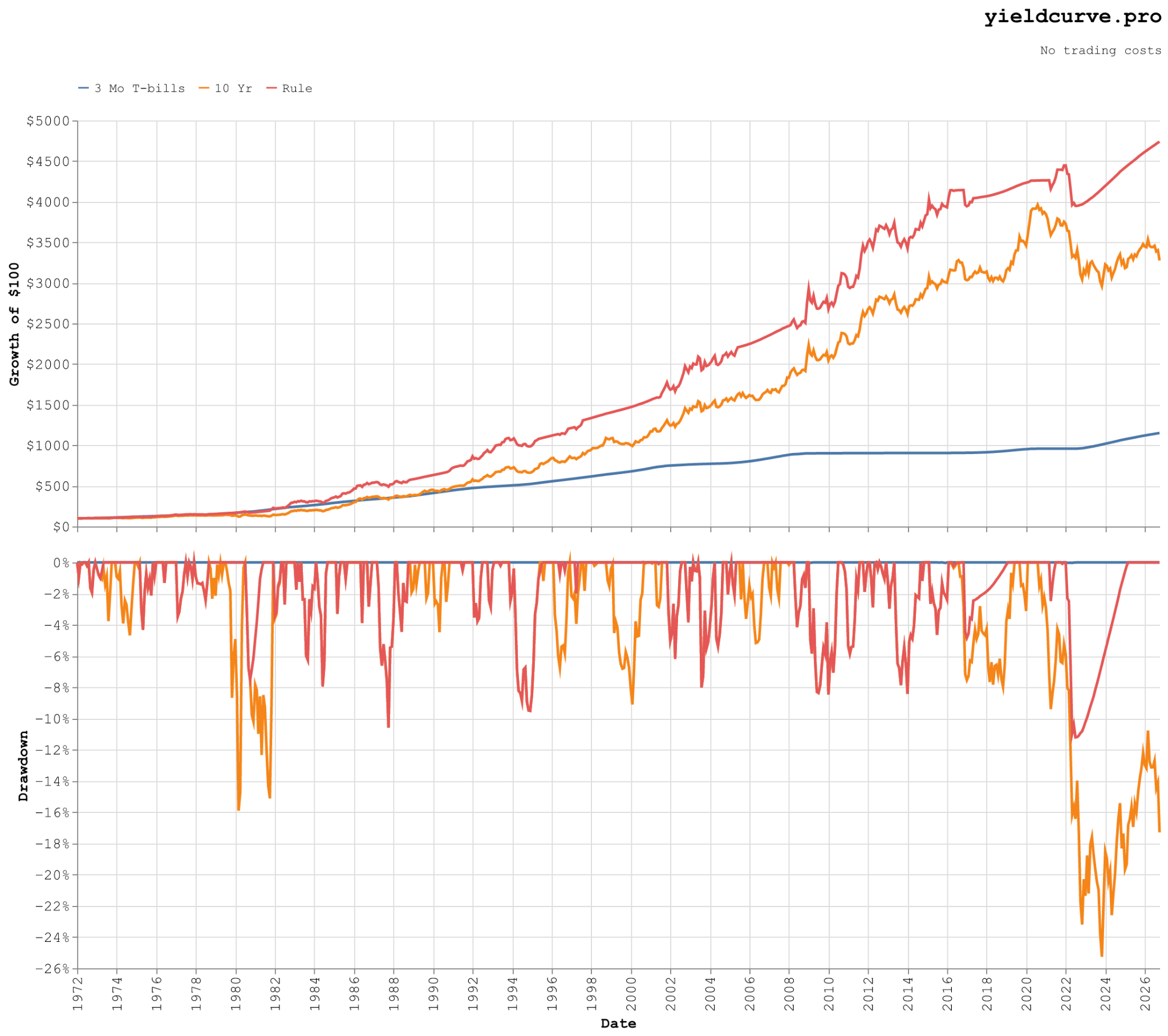
Figure 3: Growth of \$100 (top) and drawdown from the previous high (bottom) for 3 Mo T-bills, the 10 Yr and the rule, December 1971 to September 2026. Final values are \$1,150.98, \$3,276.14 and \$4,739.70.
The rule works on public data and in each half of the sample. In both halves it beat the 10 Yr with lower volatility and a smaller worst loss. Its volatility was 6.48% against 8.39% for the 10 Yr in 1972-2001, and 6.04% against 7.62% in 2001-2026. Its worst loss in the first half came in 1987. Both worst losses for the full period occurred after 2020, so they equal the 2001-2026 figures. From 2001 to 2026, the rule held the 10 Yr in 54% of months and switched 13 times, so trading costs would change the result little. The opposite rule, which holds the 10 Yr only when the spread is below its median, earned less than bills. Cambria computes its Sharpe ratio as the compounded return minus the bill return, divided by volatility. On that definition, the rule scores 0.43 from 1972 to 2026 against 0.25 for the 10 Yr, close to the paper's 0.44 and 0.22.
When Cambria published in February 2024, the rule held bills. It has held bills every month since. From March 2024 to September 2026, bills returned 12.01% and the 10 Yr returned 3.88%.
The rule's worst loss, 11.21%, ran from December 2021 to June 2022. The curve was steep at the end of 2021, so the rule held the 10 Yr into the 2022 inflation shock. A wide spread measures the premium the market offers. It does not protect against a sharp rise in yields.
The curve on September 30, 2026
Longer maturities have trailed shorter ones for five years. Over the 60 months to September 2026, the 20 Yr trailed the 2 Yr by 6.83% a year, and the 2 Yr trailed the 1 Mo bill by 2.03% a year.
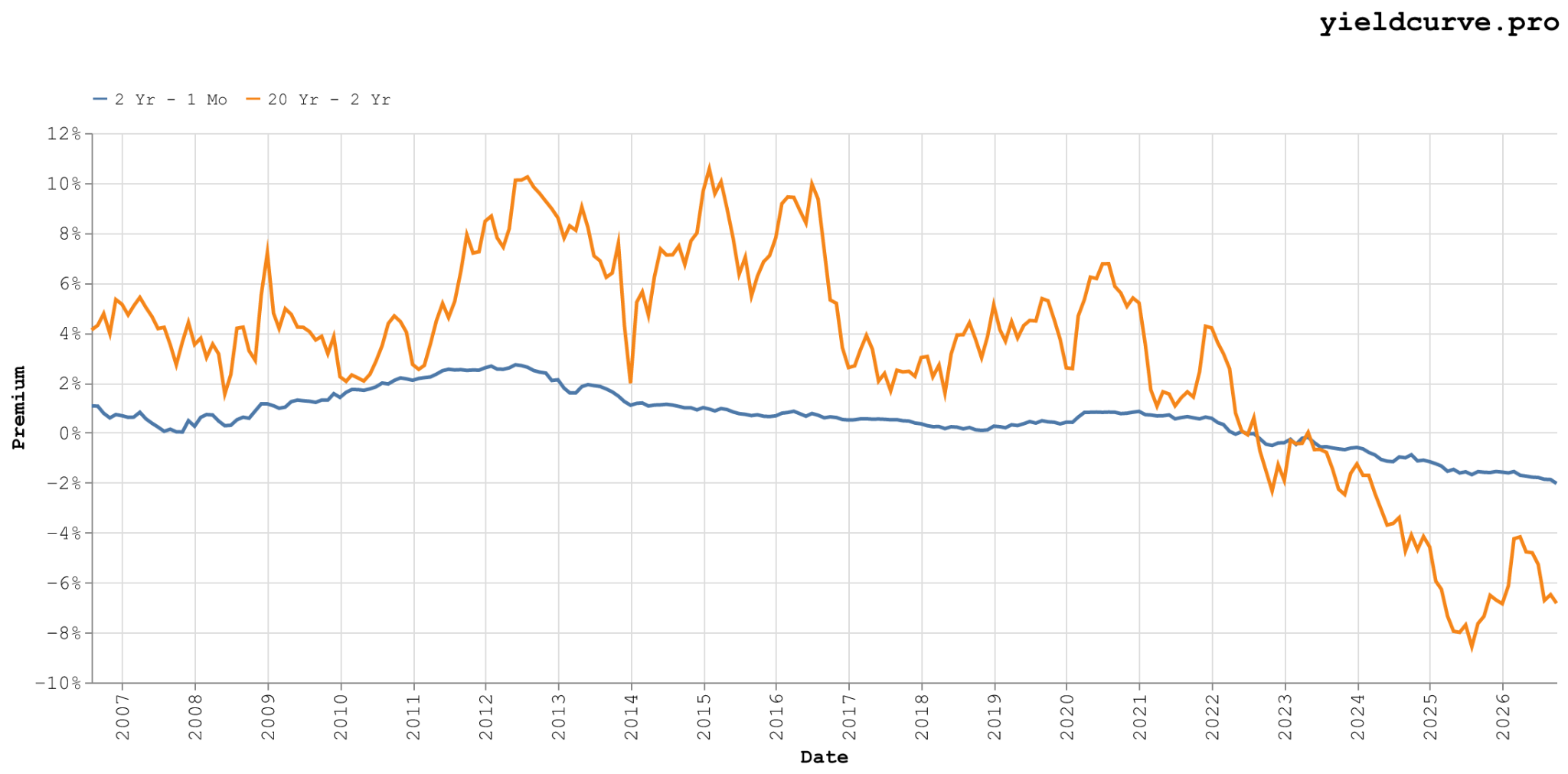
Figure 4: Average return difference over the previous 60 months, annualized, for the 2 Yr over the 1 Mo bill and the 20 Yr over the 2 Yr, July 2006 to September 2026.
Those losses have raised long yields, but a higher long yield does not by itself mean a higher premium for duration. The premium depends on the long yield minus the bill yield. The 3 Mo bill yields 4.13%, so the 10 Yr minus 3 Mo spread is 1.16 points. That is below its 1.27-point median since 1962, so the rule holds bills.
The regression also points to a below-average premium. The 20 Yr minus 1 Mo slope is 166 bp, the 41st percentile of month-start slopes since 2001. At that slope, the regression forecasts an excess return of +1.89% a year for the 20 Yr, below its +3.09% sample average. For the 5 Yr, it forecasts +1.16%, against an average of +1.66%. The 20 Yr's annual excess return varies by about 11.91 points around any forecast, so neither forecast is reliable for a single year.
Read the original series
All seven parts of Understanding the Yield Curve are free to read on yieldcurve.pro, along with the other papers in the classic papers library. Signed-in readers can ask an assistant questions about any paper in the library. Part 4, Forecasting US Bond Returns, takes up the forecasting question that the slope regression raises.


Back
Sign in to leave a comment.
Comments (0)